Visualizing Mass Spectra¶

The ms_deisotope.plot module contains several plotting functions for visualizing mass spectra using matplotlib.

A collection of tools for drawing and annotating mass spectra

import ms_deisotope
from ms_deisotope import plot
from ms_deisotope.test.common import datafile

reader = ms_deisotope.MSFileLoader(datafile("20150710_3um_AGP_001_29_30.mzML.gz"))
bunch = next(reader)

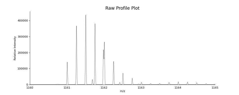
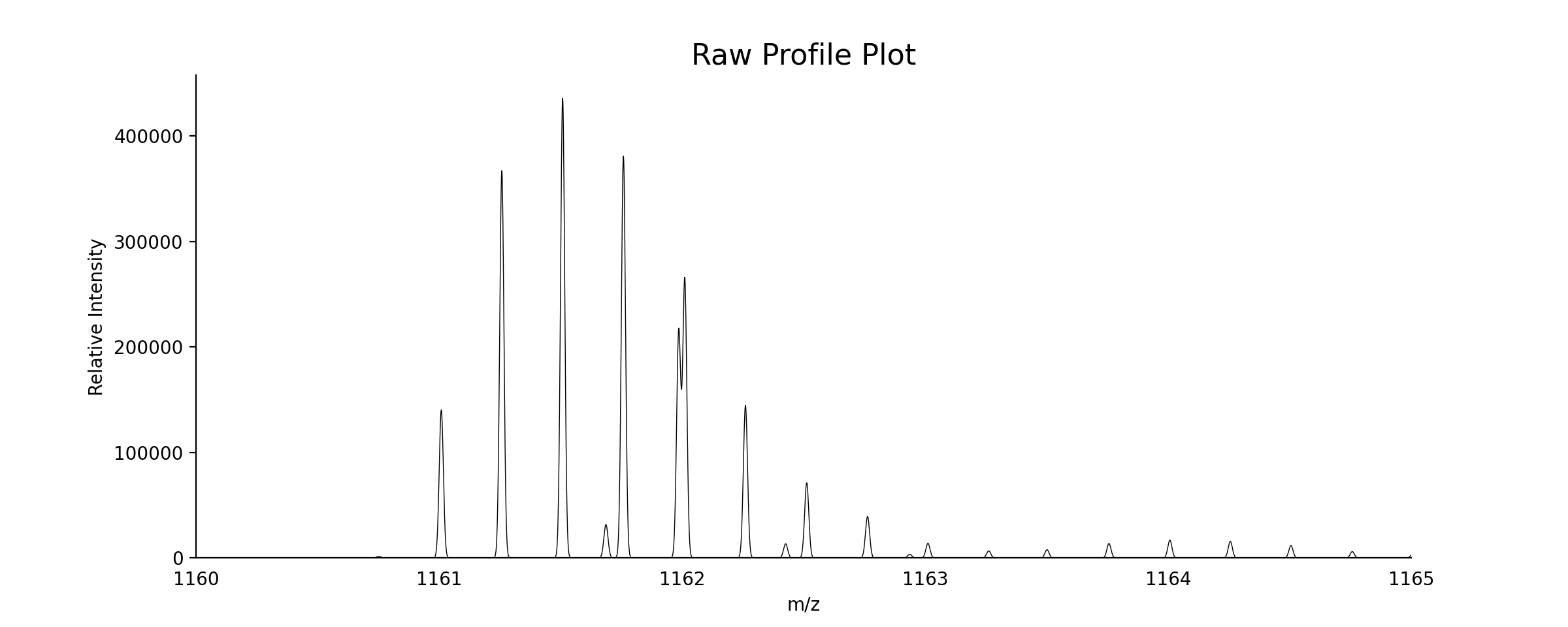
# create a profile spectrum
for peak in bunch.precursor.pick_peaks():
    peak.full_width_at_half_max = 0.02
scan = bunch.precursor.reprofile(dx=0.001)
ax = plot.draw_raw(scan.arrays, color='black', lw=0.5)
ax.set_xlim(1160, 1165)
ax.figure.set_figwidth(12)
ax.set_title("Raw Profile Plot", fontsize=16)

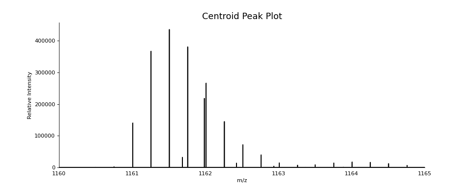
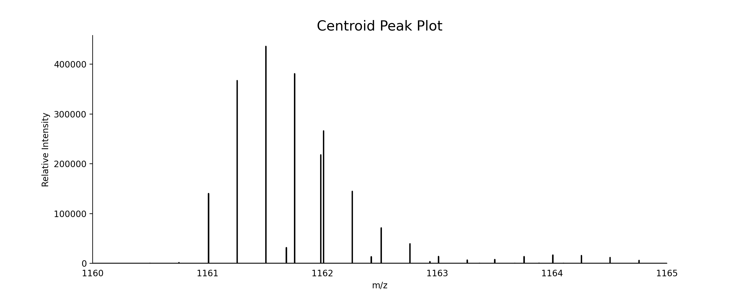
scan.pick_peaks()
ax = plot.draw_peaklist(scan.peak_set, color='black')
ax.set_xlim(1160, 1165)
ax.figure.set_figwidth(12)
ax.set_title("Centroid Peak Plot", fontsize=16)

(Source code)

(png, hires.png, pdf)¶

(png, hires.png, pdf)¶

Basic Spectrum Drawing¶

ms_deisotope.plot.draw_raw(mz_array, intensity_array=None, ax=None, normalize=False, **kwargs)[source]¶

Draws un-centroided profile data, visualizing continuous data points

Parameters

mz_array (np.ndarray or tuple) – Either the m/z array to be visualized, or if intensity_array is None, mz_array will be unpacked, looking to find a sequence of two np.ndarray objects for the m/z (X) and intensity (Y) coordinates

intensity_array (np.ndarray, optional) – The intensity array to be visualized. If None, will attempt to unpack mz_array

ax (matplotlib.Axes, optional) – The axis to draw the plot on. If missing, a new one will be created using matplotlib.pyplot.subplots()

normalize (bool, optional) – if True, will normalize the abundance dimension to be between 0 and 100%

pretty (bool, optional) – If True, will call _beautify_axes() on ax

**kwargs – Passed to matplotlib.Axes.plot()

Returns

Return type

Axes

ms_deisotope.plot.draw_peaklist(peaklist, ax=None, normalize=False, **kwargs)[source]¶

Draws centroided peak data, visualizing peak apexes.

The peaks will be converted into a single smooth curve using peaklist_to_vector().

Parameters

peaklist (Iterable of PeakLike) – The peaks to draw.

ax (matplotlib.Axes, optional) – The axis to draw the plot on. If missing, a new one will be created using matplotlib.pyplot.subplots()

normalize (bool, optional) – if True, will normalize the abundance dimension to be between 0 and 100%

pretty (bool, optional) – If True, will call _beautify_axes() on ax

**kwargs – Passed to matplotlib.Axes.plot()

Returns

Return type

matplotlib.Axes

Annotating Peaks and Envelopes¶

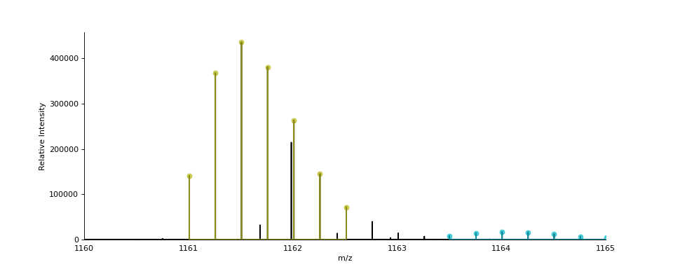
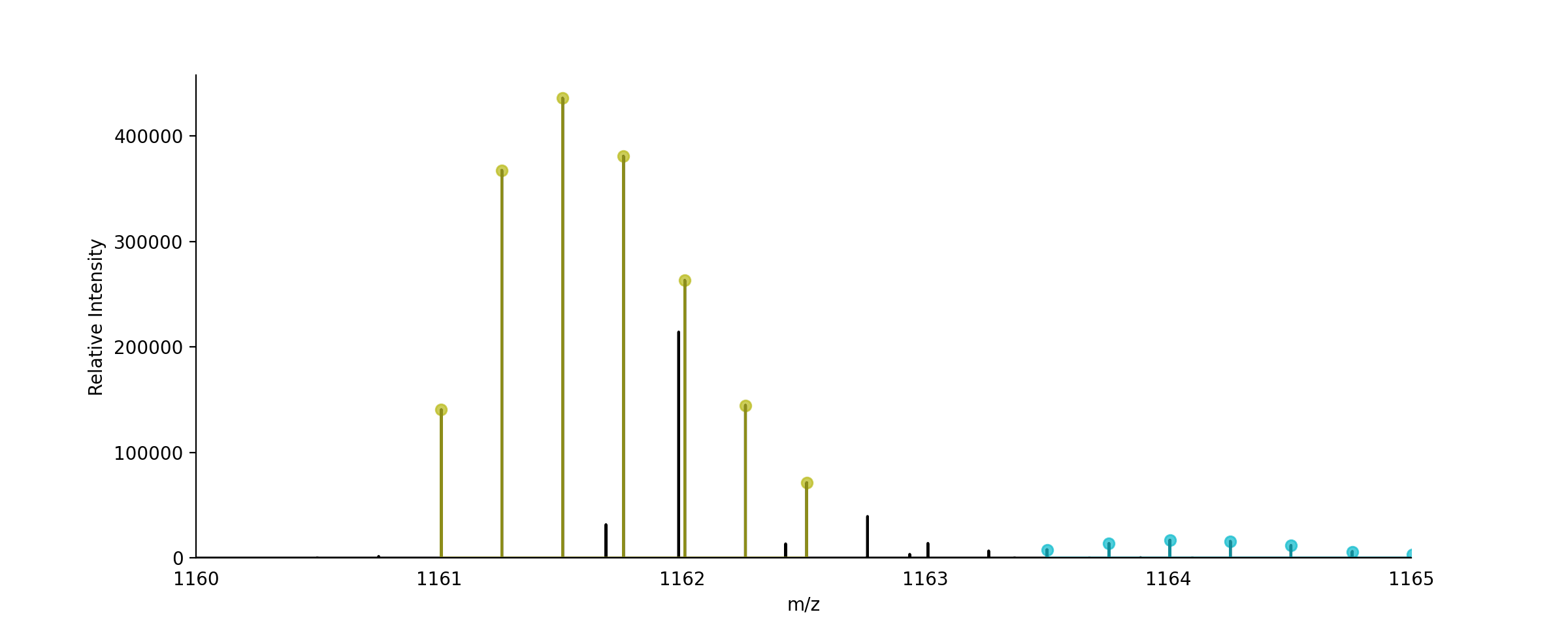
ms_deisotope.plot.annotate_isotopic_peaks(scan: ScanBase, ax: Optional[Axes] = None, color_cycle: Optional[Iterable[str]] = None, mz_range: Optional[Tuple[float, float]] = None, **kwargs)[source]¶
Mark distinct isotopic peaks from the DeconvolutedPeakSet in scan.
import ms_deisotope
from ms_deisotope import plot
from ms_deisotope.test.common import datafile

example_file = datafile("20150710_3um_AGP_001_29_30.mzML.gz")
reader = ms_deisotope.MSFileLoader(example_file)
bunch = next(reader)

bunch.precursor.pick_peaks()
bunch.precursor.deconvolute(
    scorer=ms_deisotope.PenalizedMSDeconVFitter(20., 2.0),
    averagine=ms_deisotope.glycopeptide, use_quick_charge=True)

ax = plot.draw_peaklist(bunch.precursor, color='black')
ax = plot.annotate_isotopic_peaks(bunch.precursor, ax=ax)
ax.set_xlim(1160, 1165)
ax.figure.set_figwidth(12)
(Source code, png, hires.png, pdf)

Parameters

scan (ScanBase) – The scan to annotate

ax (matplotlib._axes.Axes) – An Axes object to draw the plot on

color_cycle (Iterable) – An iterable to draw isotopic cluster colors from

mz_range ((float, float), optional) – The m/z range to annotate peaks within. Defaults to the full range if not specified.

Returns

Return type

matplotlib._axes.Axes
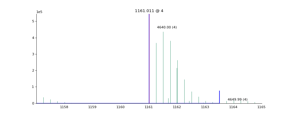
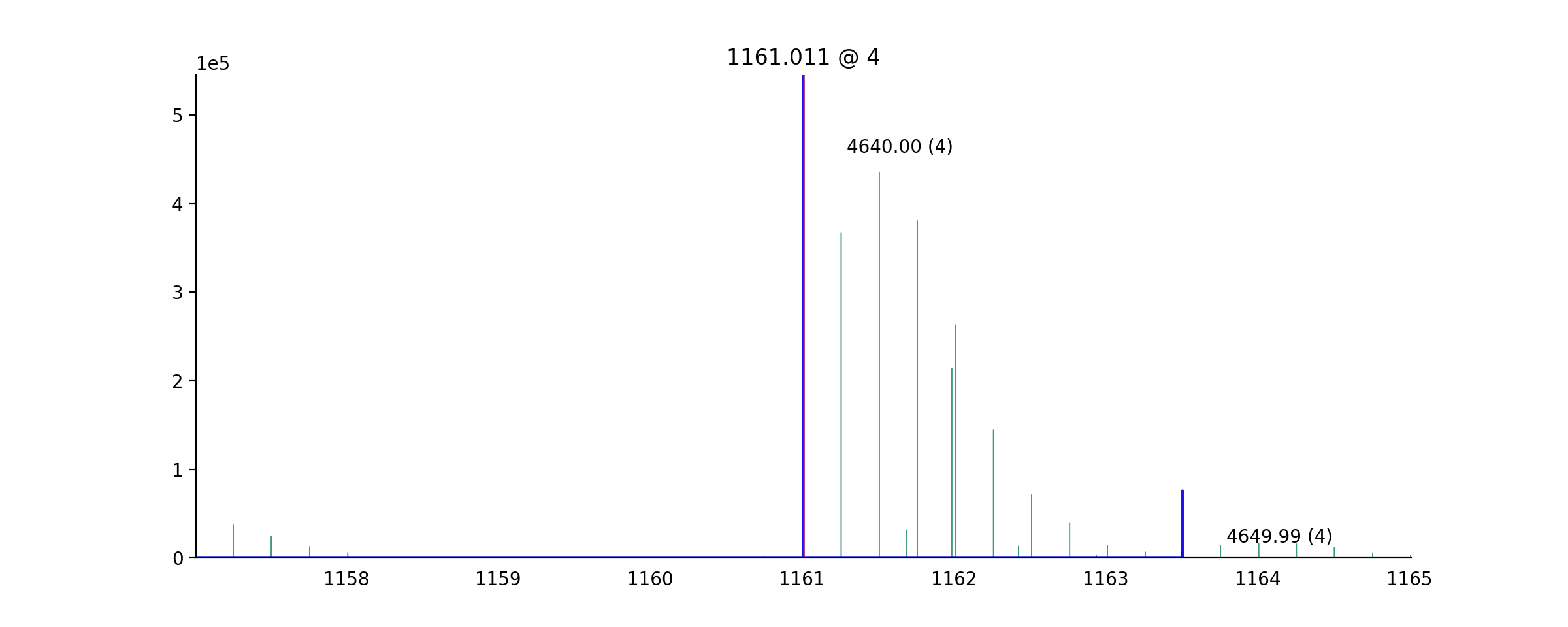
ms_deisotope.plot.label_peaks(scan: ScanBase, min_mz: Optional[float] = None, max_mz: Optional[float] = None, ax: Optional[Axes] = None, is_deconvoluted: Optional[bool] = None, threshold: Optional[float] = None, **kwargs)[source]¶

Label a region of the peak list, marking centroids with their m/z or mass. If the peaks of scan have been deconvoluted, the most abundant peak will be annotated with “<neutral mass> (<charge>)”, otherwise just “<m/z>”.

Parameters

scan (ScanBase) – The scan to annotate

min_mz (float, optional) – The minimum m/z to annotate

max_mz (float, optional) – The maximum m/z to annotate

ax (matplotlib._axes.Axes) – An Axes object to draw the plot on

is_deconvoluted (bool, optional) – Whether or not to always use Scan.deconvoluted_peak_set

threshold (float, optional) – The intensity threshold under which peaks will be ignored

Returns

ax (matplotlib._axes.Axes) – The axes the plot was drawn on

annotations (list of matplotlib.text.Text) – The list of matplotlib.text.Text annotations
ms_deisotope.plot.annotate_scan_single(scan: ScanBase, product_scan: ScanBase, ax: Optional[Axes] = None, label: bool = True, standalone=True) → Axes[source]¶
Draw a zoomed-in view of the MS1 spectrum scan surrounding the area around each precursor ion that gave rise to product_scan with monoisotopic peaks and isolation windows marked.
import ms_deisotope
from ms_deisotope import plot
from ms_deisotope.test.common import datafile

example_file = datafile("20150710_3um_AGP_001_29_30.mzML.gz")

reader = ms_deisotope.MSFileLoader(example_file)
bunch = next(reader)

bunch.precursor.pick_peaks()
bunch.precursor.deconvolute(
    scorer=ms_deisotope.PenalizedMSDeconVFitter(20., 2.0),
    averagine=ms_deisotope.glycopeptide, use_quick_charge=True)

ax = plot.annotate_scan_single(bunch.precursor, bunch.products[0])
ax.figure.set_figwidth(12)
(Source code, png, hires.png, pdf)

Parameters

scan (ScanBase) – The MS1 scan to annotate

product_scan (ScanBase) – The product scan to annotate the precursor ion of

ax (matplotlib._axes.Axes) – An Axes object to draw the plot on

Returns

Return type

matplotlib._axes.Axes
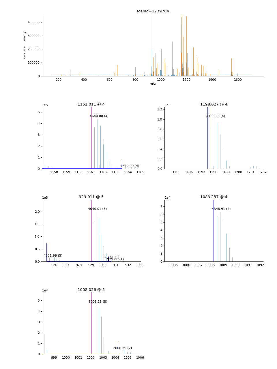
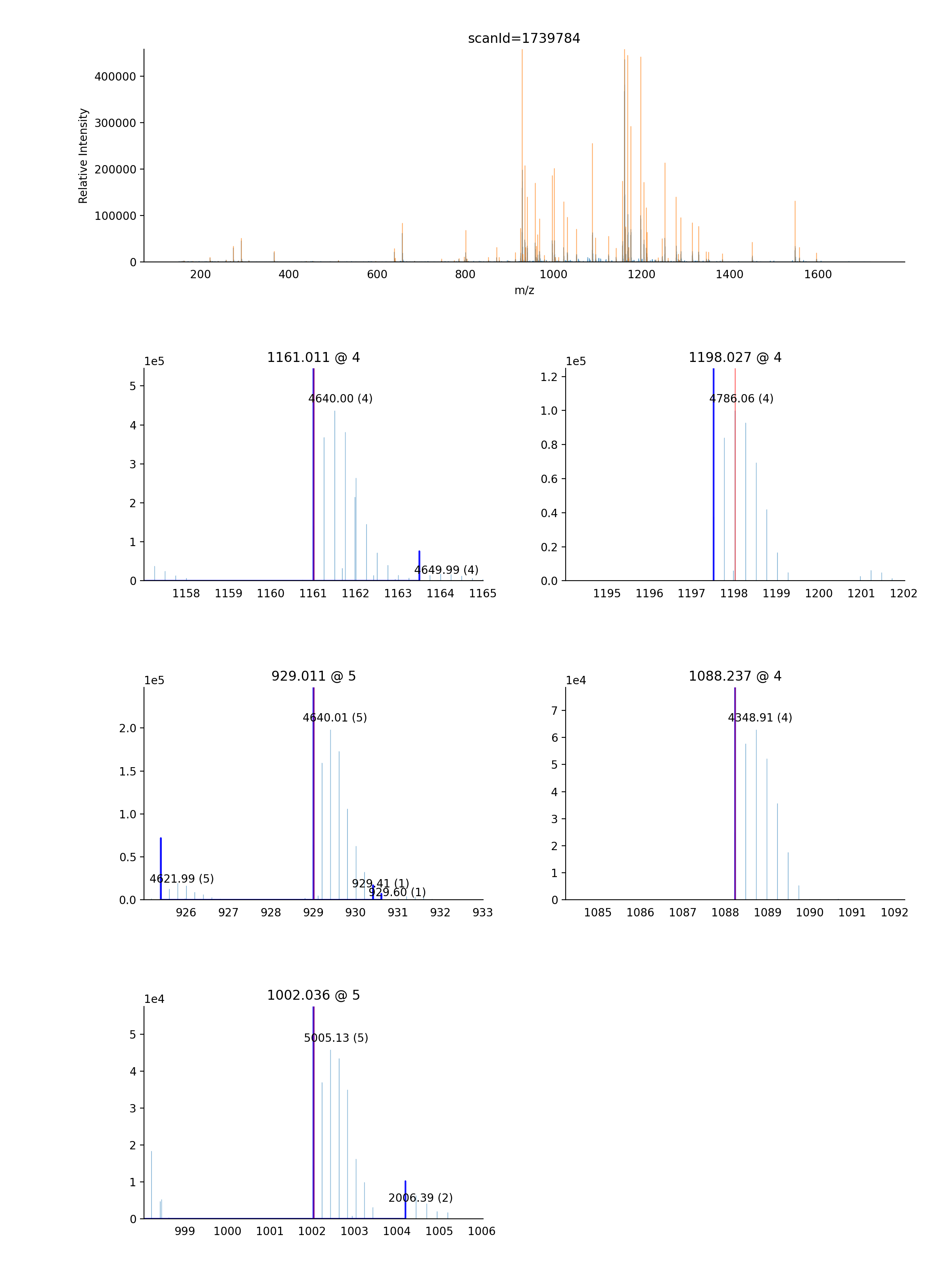
ms_deisotope.plot.annotate_scan(scan: ScanBase, products: Sequence[ScanBase], nperrow: int = 4, ax: Optional[Axes] = None, label: bool = True) → Axes[source]¶
Given an MS1 ScanBase scan and a Sequence of ScanBase product scans, draw the MS1 spectrum in full profile, and then in a subplot grid below it, draw a zoomed-in view of the MS1 spectrum surrounding the area around each precursor ion that gave rise to the scans in products, with monoisotopic peaks and isolation windows marked.
import ms_deisotope
from ms_deisotope import plot
from ms_deisotope.test.common import datafile

example_file = datafile("20150710_3um_AGP_001_29_30.mzML.gz")

reader = ms_deisotope.MSFileLoader(example_file)
bunch = next(reader)

bunch.precursor.pick_peaks()
bunch.precursor.deconvolute(
    scorer=ms_deisotope.PenalizedMSDeconVFitter(20., 2.0),
    averagine=ms_deisotope.glycopeptide, use_quick_charge=True)

ax = plot.annotate_scan(bunch.precursor, bunch.products, nperrow=2)
ax.figure.set_figwidth(12)
ax.figure.set_figheight(16)
(Source code, png, hires.png, pdf)

Parameters

scan (ScanBase) – The precursor MS1 scan

products (Sequence of ScanBase) – The collection of MSn scans based upon scan

nperrow (int) – The number of precursor ion subplots to draw per row of the grid. Defaults to 4.

ax (matplotlib._axes.Axes) – An Axes object to use to find the figure to draw the plot on.

Returns

The axes of the full MS1 profile plot

Return type

matplotlib._axes.Axes